How YOLO works?
Overview
This tutorial would show a basic explanation on how YOLO works using Tensorflow. The code for this tutorial is designed to run on Python and Tensorflow. It can be found in it’s entirety at this Github repo1.
What is YOLO?
YOLO stands for You Only Look Once. It’s an object detector that uses features learned by a deep convolutional neural network to detect an object.
The main core concept of YOLO is to use a single neural network to predict bounding boxes and class probabilities directly from full images in one evaluation. Since the whole detection pipeline is a single network, it can be optimized end-to-end directly on detection performance
Performance
Base network runs at 45frames per second with no batch processing on a Titan X GPU and a fast version runs at more than 150 fps. Furthermore, YOLO achieves more than twice the mean average precision of other real-time systems of its time.
How it works
This system is based in residual blocks, bounding box regression, and IOU techniques.
Residual Blocks divides the input image into an S × S grid. If the center of an object falls into a grid cell, that grid cell is responsible for detecting that object.
Example, Inception actually produces an 8x8x2048 representation before using average pooling to bring this to 1x1x2048. We can interpret the 8x8x2048 representation as a grid of features, breaking the image down into 8 horizontal and 8 vertical grid squares. Then, instead of mapping one 2048-dimensional vector to the class labels, we can use a 1×1 convolution to map each one of these vectors to a class label, giving us a prediction at the cell level.
The image below shows the resulting grid. The edges of the image are not covered: this is our attempt to take Inception’s lack of padding in its convolutional layers into account. The grid cells predicting pedestrians with a probability greater than 0.5 are drawn in green.
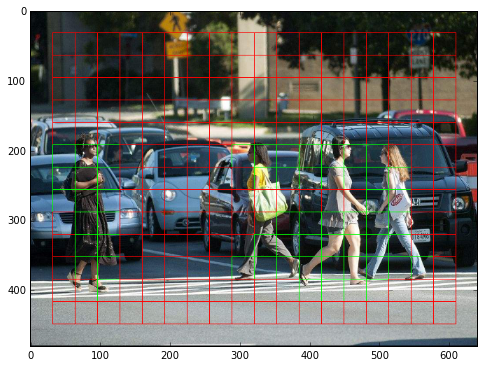
You will notice the image is bigger than 299×299. This is a nice property of the Inception architecture: as it is fully convolutional, it can be fed with any size of input image. In our case, we used 640×480 as an input, which produces the 13x18x2048 feature grid shown.
IOU - Each grid cell predicts B bounding boxes and confidence scores for those boxes. If object exists in that cell, the confidence scores should be zero. Otherwise we want the confidence score to equal the intersection over union (IOU) between the predicted box and the ground truth.
bounding box regression- YOLO uses a single regression module to predict: x, y, w, h, and confidence.
- The (x, y) coordinates represent the center of the box relative to the bounds of the grid cell.
- The width and height are predicted relative to the whole image.
- Finally the confidence prediction represents the IOU between the predicted box and any ground truth box.
This method can be applyed to the example above but instead of predicting a class probability at each cell (13x18x2048 grid), it predicts four numbers: the dimensions of the bounding box of the object under its grid cell. Training then works as follows.
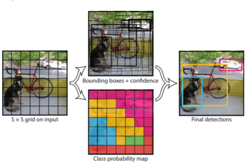
As the image above shows, YOLO algorithm divides the image into an S × S grid and for each grid cell predicts B bounding boxes, confidence for those boxes, and C class probabilities. These predictions are encoded as S × S × (B ∗ 5 + C) tensor.
Training
YOLO normalizes the bounding box width and height by the image width and height so that they fall between 0 and 1. The bounding box x and y coordinates to be offsets of a particular grid cell location are also bounded between 0 and 1.
Bellow is a snippet code of the loss function for YOLO v1. As you can see there is a loss function for every tensor.
        # loss function
        self.subX = tf.subtract(boxes0, self.x_)
        self.subY = tf.subtract(boxes1, self.y_)
        self.subW = tf.subtract(tf.sqrt(tf.abs(boxes2)), tf.sqrt(self.w_))
        self.subH = tf.subtract(tf.sqrt(tf.abs(boxes3)), tf.sqrt(self.h_))
        self.subC = tf.subtract(scales, self.C_)
        self.subP = tf.subtract(class_probs, self.p_)
        self.lossX = tf.multiply(self.lambdacoord, tf.reduce_sum(tf.multiply(self.obj, tf.multiply(self.subX, self.subX)), axis=[1, 2, 3]))
        self.lossY = tf.multiply(self.lambdacoord, tf.reduce_sum(tf.multiply(self.obj, tf.multiply(self.subY, self.subY)), axis=[1, 2, 3]))
        self.lossW = tf.multiply(self.lambdacoord, tf.reduce_sum(tf.multiply(self.obj, tf.multiply(self.subW, self.subW)), axis=[1, 2, 3]))
        self.lossH = tf.multiply(self.lambdacoord, tf.reduce_sum(tf.multiply(self.obj, tf.multiply(self.subH, self.subH)), axis=[1, 2, 3]))
        self.lossCObj = tf.reduce_sum(tf.multiply(self.obj, tf.multiply(self.subC, self.subC)), axis=[1, 2, 3])
        self.lossCNobj = tf.multiply(self.lambdanoobj, tf.reduce_sum(tf.multiply(self.noobj, tf.multiply(self.subC, self. subC)), axis=[1, 2, 3]))
        self.lossP = tf.reduce_sum(tf.multiply(self.objI,tf.reduce_sum(tf.multiply(self.subP, self.subP), axis=3)), axis= [1,2])
        self.loss = tf.add_n((self.lossX, self.lossY, self.lossW, self.lossH, self.lossCObj, self.lossCNobj, self.lossP))
        self.loss = tf.reduce_mean(self.loss)
To maximize parallel computation speed I will be using a constant input size (all images of fixed height and width.)
Limitations of YOLO
Reference
Source Code: dshahrokhian repository [1]
You Only Look Once: Unified, Real-Time Object Detection [2]