Regression of object bounding box (localization)
Overview
I would like to present a practical and yet powerful explanation on the foundations for today’s state of the art object detection in deep neural networks (DNN).
Localization
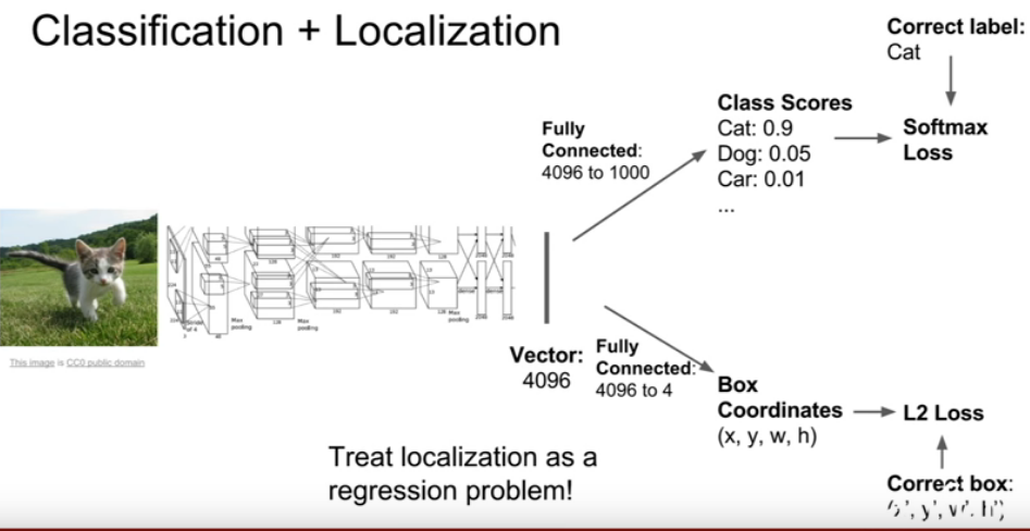
Regression of object bounding box in theory the basic foundation of the State-of-the-art approaches as shown on Pascal VOC. DNN-based regression algorithms are capable of learning features. Similar to classification we can use regression to capture geometric information (localization). This can be done as simple as replace the last layer favorite CNN classification architecture and with a regression layer to capture object locations (bounding boxes parameters). You can picture this step as replacing your softmax classifier with a regression layer with the parameters of the network and total number of pixels to generates an object binary mask DNN.
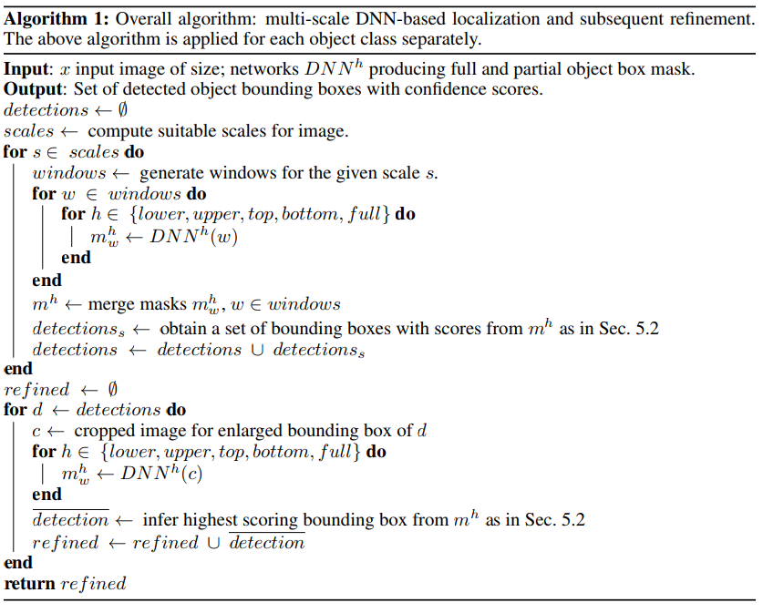
Based on this regression model, we can generate masks for the full object as well as portions of the object. A single DNN regression can give us masks of multiple objects in an image. To further increase the precision of localization, DNN localizer can be applied in conjunction with number of other algorithms. The following implementation is my briefly explanation of Google’s early on application of localization on small set of large subwindows [1].
Masking
Since the output of the network has a fixed dimension, we can predict a mask of a fixed size N = d × d. After being resized to the image size, the resulting binary mask represents one or several objects: it should have value 1 at particular pixel if this pixel lies within the bounding box of an object of a given class and 0 otherwise. The network is trained by minimizing the L2 error for predicting a ground truth mask.
Multiple Images detection
To deal with multiple objects, several masks can be implemented to represent either the full object or part of it. Since our end goal is to produce a bounding box, we can use one network to predict the object box mask and four additional networks to predict four halves of the box: bottom, top, left and right halves, all denoted by mh , h ∈ {full, bottom, top, left, left}. These five predictions are over-complete but help reduce uncertainty and deal with mistakes in some of the masks. Further, if two objects of the same type are placed next to each other, then at least two of the produced five masks would not have the objects merged which would allow to disambiguate them. This would enable the detection of multiple objects.
At training time, we need to convert the object box to these five masks. Since the masks can be much smaller than the original image, we need to downsize the ground truth mask to the size of the network output. Denote by T(i, j) the rectangle in the image for which the presence of an object is predicted by output (i, j) of the network. This rectangle overlap coparation of the size of the output mask and the height and width of the image.
During training we assign as value m(i, j) to be predicted as portion of T(i, j) being covered by box bb(h) :
mh(i, j) = area(bb(h) ∩ T(i, j)) / area(T(i, j))
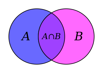
where bb(full) corresponds to the ground truth object box. For the remaining values of h, bb(h) corresponds to the four halves of the original box.
This is not a sliding window
Note that it is quite different from sliding window approaches because localization with be computed by a small number of windows per image, usually less than 40. The goal is to generated object masks at each scale are merged by maximum operation. Consider 10 bounding boxes with mean dimension equal to [0.1, . . . , 0.9] of the mean image dimension.
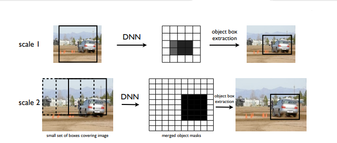
The generated object masks at each scale are merged by maximum operation. This gives us three masks of the size of the image, each ‘looking’ at objects of different sizes. For each scale, we apply the bounding box inference to arrive at a set of detections.
Improve localization
To further improve the localization, we go through a second stage of DNN regression called refinement. The DNN localizer is applied on the windows defined by the initial detection stage – each of the 15 bounding boxes is enlarged by a factor of 1.2 and is applied to the network. Applying the localizer at higher resolution increases the precision of the detections significantly.
Other applications with Localization
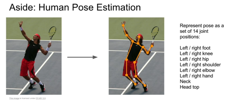
Localization can be implemented for many different problems. The concept of tuning parameters with regression models is what makes machine learning a revolutionary tool. Take a look at the image bellow. You can use localization to keep track of body joins.
Reference
Deep Neural Networks for Object Detection
ImageNet Classification with Deep Convolutional Neural Networks
| Justin Johnson [Lecture 11 | Detection and Segmentation] |