advanced optimizers
TensorFlow Optimizers
TensorFlow Optimizer base class provides methods to compute gradients for a loss and apply gradients to variables. This practicle guide to demonstrate how popular optimization algorithms used for training neural networks perform in a Convolutional Neural Network (CNN) trained on MNIST dataset.
**NOTE: Adaptive optimization methods(AdaGrad, RMSProp, and Adam), which perform local optimization with a metric constructed from the history of iterates, are becoming increasingly popular for training deep neural networks. But in some cases it has been demontrated that for simple overparameterized problems, adaptive methods underperfome gradient descent (GD) or stochastic gradient descent (SGD). Even though Adaptive optimizers solutions have better training performance it does not mean that results will generalize that well. [[5]]
Stochastic Gradient Descent
Stochastic Gradient Descent (SGD) updates parameters in the negative direction of the gradient. The learning rate parameter $\epsilon_k$ should be decreased over time. SGD computation time is proportional to mini-batch size $m$:
\begin{eqnarray}
g &=& \frac{1}{m}\nabla_\theta \sum_i L(f(x^{(i)};\theta), y^{(i)})
\theta &=& \theta - \epsilon_k \times g
\end{eqnarray}
Momentum
Momentum accumulates exponentially decaying moving average of past gradients and continues to move in their direction. It simply adds a fraction of the previous step to a current step direciton. This achieves amplification of speed in the correct dirrection and softens oscillation in wrong directions. Step size depends on how large and how aligned the sequence of gradients are, common values of momentum parameter $\alpha$ are 0.5 and 0.9.
Learning rate: In the beginning of learning a big momentum will only hinder your progress, so it makse sense to use something like 0.01 and once all the high gradients disappeared you can use a bigger momentom.
Challenges: There is one problem with momentum: when we are very close to the goal, our momentum in most of the cases is very high and it does not know that it should slow down. This can cause it to miss or oscillate around the minima
\begin{eqnarray}
v &=& \alpha v - \epsilon \nabla_\theta \big(\frac{1}{m}\sum_i
L(f(x^{(i)};\theta), y^{(i)}) \big)
\theta &=& \theta + v
\end{eqnarray}
Nesterov Momentum
Nesterov Momentum inspired by Nesterov’s accelerated gradient method. Nesterov’s momentum the gradient is evaluated after the current velocity is applied, thus Nesterov’s momentum adds a correction factor to the gradient.
In momentum we first compute gradient and then make a jump in that direction amplified by whatever momentum we had previously. NAG does the same thing but in another order: at first we make a big jump based on our stored information, and then we calculate the gradient and make a small correction. This seemingly irrelevant change gives significant practical speedups:
\begin{eqnarray}
v &=& \alpha v - \epsilon \nabla_\theta \big(\frac{1}{m}\sum_i
L(f(x^{(i)};\theta + \alpha \times v), y^{(i)}) \big)
\theta &=& \theta + v
\end{eqnarray}
AdaGrad
AdaGrad adapts the learning rates of all model parameters, learning rate is inversely proportional to the square root of the sum of historical squared values.
Use case: It performs larger updates for infrequent parameters and smaller updates for frequent one. Because of this it is well suited for sparse data (NLP or image recognition).
Advantage: Another advantage is that it basically illiminates the need to tune the learning rate. Weights that receive high gradients will have their effective learning rate reduced, while weights that receive small or infrequent updates will have their effective learning rate increased.
Challenges: This causes the biggest problem: at some point of time the learning rate is so small that the system stops learning
\begin{eqnarray}
g &=& \frac{1}{m}\nabla_\theta \sum_i L(f(x^{(i)};\theta), y^{(i)})
s &=& s + g^{T}g
\theta &=& \theta - \epsilon_k \times g / \sqrt{s+eps}
\end{eqnarray}
RMSProp
RMSProp resolves the problem of monotonically decreasing learning rate. In RMSProp the learning rate is calculated approximately as one divided by the sum of square roots. At each stage you add another square root to the sum (exponential weighted moving average), which causes denominator to constantly decrease. In RMSProp instead of summing all past square roots it uses sliding window which discards history from the extreme past.
use case: RMSProp has been shown to be an effective and practical optimization algorithm for deep neural networks:
\begin{eqnarray}
g &=& \frac{1}{m}\nabla_\theta \sum_i L(f(x^{(i)};\theta), y^{(i)})
s &=& \mathrm{decay_rate}\times s + (1-\mathrm{decay_rate}) g^{T}g
\theta &=& \theta - \epsilon_k \times g / \sqrt{s+eps}
\end{eqnarray}
Adam
Adam derives from “adaptive moments”, it can be seen as a variant on the combination of RMSProp and momentum but in addition to storing learning rates for each of the parameters it also stores momentum changes for each of them separately. The update looks like RMSProp except that a smooth version of the gradient is used instead of the raw stochastic gradient, the full adam update also includes a bias correction mechanism, recommended values in the paper are $\epsilon = 1e-8$, $\beta_1 = 0.9$, $\beta_2 = 0.999$:
\begin{eqnarray}
g &=& \frac{1}{m}\nabla_\theta \sum_i L(f(x^{(i)};\theta), y^{(i)})
m &=& \beta_1 m + (1-\beta_1) g
s &=& \beta_2 v + (1-\beta_2) g^{T}g
\theta &=& \theta - \epsilon_k \times m / \sqrt{s+eps}
\end{eqnarray}
Examples:
Let’s examing the performance of different optimizers using TensorFlow!
%matplotlib inline

import numpy as np
import tensorflow as tf
from tensorflow.examples.tutorials.mnist import input_data
from tensorflow.contrib.layers import variance_scaling_initializer

import seaborn as sns
import matplotlib.pyplot as plt
Let’s define the auxiliary functions that will help us define the neural network.
def weight_variable(name, shape):
    he_normal = variance_scaling_initializer(factor=2.0, mode='FAN_IN', uniform=False,
                                             seed=None, dtype=tf.float32)
    return tf.get_variable(name, shape=shape, initializer=he_normal)

def bias_variable(shape):
    initial = tf.constant(0.1, shape=shape)
    return tf.Variable(initial)

def conv2d(x, W):
    return tf.nn.conv2d(x, W, strides=[1,1,1,1], padding='SAME')

def max_pool_2x2(x):
    return tf.nn.max_pool(x, ksize=[1,2,2,1], strides=[1,2,2,1], padding='SAME')
We use the recommended He normal initialization together with ReLU activation functions.
#dataset
mnist = input_data.read_data_sets("./MNIST_data/", one_hot=True)

#parameters
learning_rate = 0.001
training_epochs = 1000
batch_size = 50
display_step = 100
Successfully downloaded train-images-idx3-ubyte.gz 9912422 bytes.
Extracting ./MNIST_data/train-images-idx3-ubyte.gz
Successfully downloaded train-labels-idx1-ubyte.gz 28881 bytes.
Extracting ./MNIST_data/train-labels-idx1-ubyte.gz
Successfully downloaded t10k-images-idx3-ubyte.gz 1648877 bytes.
Extracting ./MNIST_data/t10k-images-idx3-ubyte.gz
Successfully downloaded t10k-labels-idx1-ubyte.gz 4542 bytes.
Extracting ./MNIST_data/t10k-labels-idx1-ubyte.gz
Let’s define our computational graph.
x = tf.placeholder(tf.float32, [None, 784])
y_= tf.placeholder(tf.float32, [None, 10])
x_image = tf.reshape(x, [-1,28,28,1])

#layer 1
W_conv1 = weight_variable("W1", [5,5,1,32])
b_conv1 = bias_variable([32])
h_conv1 = tf.nn.relu(conv2d(x_image, W_conv1) + b_conv1)
h_pool1 = max_pool_2x2(h_conv1)

#layer 2
W_conv2 = weight_variable("W2", [5,5,32,64])
b_conv2 = bias_variable([64])
h_conv2 = tf.nn.relu(conv2d(h_pool1, W_conv2) + b_conv2)
h_pool2 = max_pool_2x2(h_conv2)

#layer 3
W_fc1 = weight_variable("W3", [7*7*64, 1024])
b_fc1 = bias_variable([1024])
h_pool2_flat = tf.reshape(h_pool2, [-1,7*7*64])
h_fc1 = tf.nn.relu(tf.matmul(h_pool2_flat, W_fc1) + b_fc1)

#dropout
keep_prob = tf.placeholder(tf.float32)
h_fc1_drop = tf.nn.dropout(h_fc1, keep_prob)

#layer 5
W_fc2 = weight_variable("W5", [1024, 10])
b_fc2 = bias_variable([10])
y_conv = tf.matmul(h_fc1_drop, W_fc2) + b_fc2

cross_entropy = tf.reduce_mean(tf.nn.softmax_cross_entropy_with_logits(labels=y_, logits=y_conv))
We’ll focus on the following optimizers:
#optimizers
train_step1 = tf.train.GradientDescentOptimizer(learning_rate).minimize(cross_entropy)
train_step2 = tf.train.MomentumOptimizer(learning_rate, momentum=0.9, use_nesterov=True).minimize(cross_entropy)
train_step3 = tf.train.RMSPropOptimizer(learning_rate).minimize(cross_entropy)
train_step4 = tf.train.AdamOptimizer(learning_rate).minimize(cross_entropy)
correct_prediction = tf.equal(tf.argmax(y_conv,1), tf.argmax(y_,1))
accuracy = tf.reduce_mean(tf.cast(correct_prediction, tf.float32))

init = tf.global_variables_initializer()
Let’s evaluate each optimizer one by one:
with tf.Session() as sess1:
    sess1.run(init)

    print "training with SGD optimizer..."
    avg_loss_sgd = np.zeros(training_epochs)
    for epoch in range(training_epochs):
        batch_xs, batch_ys = mnist.train.next_batch(batch_size)

        _, loss = sess1.run([train_step1, cross_entropy],
                            feed_dict={x: batch_xs, y_: batch_ys, keep_prob: 0.5})
        avg_loss_sgd[epoch] = loss

        if epoch % display_step == 0:
            train_accuracy = accuracy.eval(feed_dict={x:batch_xs, y_:batch_ys, keep_prob: 1.0})
            print("Epoch %04d, training accuracy %.2f"%(epoch, train_accuracy))
    #end for
    print("test accuracy %g" %accuracy.eval(feed_dict={x: mnist.test.images, y_: mnist.test.labels, keep_prob: 1.0}))
training with SGD optimizer...
Epoch 0000, training accuracy 0.10
Epoch 0100, training accuracy 0.70
Epoch 0200, training accuracy 0.88
Epoch 0300, training accuracy 0.80
Epoch 0400, training accuracy 0.90
Epoch 0500, training accuracy 0.82
Epoch 0600, training accuracy 0.94
Epoch 0700, training accuracy 0.92
Epoch 0800, training accuracy 0.80
Epoch 0900, training accuracy 0.94
test accuracy 0.9084
with tf.Session() as sess2:
    sess2.run(init)

    print "training with momentum optimizer..."
    avg_loss_momentum = np.zeros(training_epochs)
    for epoch in range(training_epochs):
        batch_xs, batch_ys = mnist.train.next_batch(batch_size)

        _, loss = sess2.run([train_step2, cross_entropy],
                            feed_dict={x: batch_xs, y_: batch_ys, keep_prob: 0.5})
        avg_loss_momentum[epoch] = loss

        if epoch % display_step == 0:
            train_accuracy = accuracy.eval(feed_dict={x:batch_xs, y_:batch_ys, keep_prob: 1.0})
            print("Epoch %04d, training accuracy %.2f"%(epoch, train_accuracy))
    #end for
    print("test accuracy %g" %accuracy.eval(feed_dict={x: mnist.test.images, y_: mnist.test.labels, keep_prob: 1.0}))
training with momentum optimizer...
Epoch 0000, training accuracy 0.14
Epoch 0100, training accuracy 0.88
Epoch 0200, training accuracy 0.94
Epoch 0300, training accuracy 0.90
Epoch 0400, training accuracy 0.96
Epoch 0500, training accuracy 0.96
Epoch 0600, training accuracy 0.94
Epoch 0700, training accuracy 0.94
Epoch 0800, training accuracy 0.96
Epoch 0900, training accuracy 0.98
test accuracy 0.9662
with tf.Session() as sess3:
    sess3.run(init)

    print "training with RMSProp optimizer..."
    avg_loss_rmsprop = np.zeros(training_epochs)
    for epoch in range(training_epochs):
        batch_xs, batch_ys = mnist.train.next_batch(batch_size)

        _, loss = sess3.run([train_step3, cross_entropy],
                            feed_dict={x: batch_xs, y_: batch_ys, keep_prob: 0.5})
        avg_loss_rmsprop[epoch] = loss

        if epoch % display_step == 0:
            train_accuracy = accuracy.eval(feed_dict={x:batch_xs, y_:batch_ys, keep_prob: 1.0})
            print("Epoch %04d, training accuracy %.2f"%(epoch, train_accuracy))
    #end for
    print("test accuracy %g" %accuracy.eval(feed_dict={x: mnist.test.images, y_: mnist.test.labels, keep_prob: 1.0}))
training with RMSProp optimizer...
Epoch 0000, training accuracy 0.06
Epoch 0100, training accuracy 0.90
Epoch 0200, training accuracy 1.00
Epoch 0300, training accuracy 1.00
Epoch 0400, training accuracy 1.00
Epoch 0500, training accuracy 1.00
Epoch 0600, training accuracy 0.98
Epoch 0700, training accuracy 1.00
Epoch 0800, training accuracy 1.00
Epoch 0900, training accuracy 1.00
test accuracy 0.9793
with tf.Session() as sess4:
    sess4.run(init)

    print "training with Adam optimizer..."
    avg_loss_adam = np.zeros(training_epochs)
    for epoch in range(training_epochs):
        batch_xs, batch_ys = mnist.train.next_batch(batch_size)

        _, loss = sess4.run([train_step4, cross_entropy],
                            feed_dict={x: batch_xs, y_: batch_ys, keep_prob: 0.5})
        avg_loss_adam[epoch] = loss

        if epoch % display_step == 0:
            train_accuracy = accuracy.eval(feed_dict={x:batch_xs, y_:batch_ys, keep_prob: 1.0})
            print("Epoch %04d, training accuracy %.2f"%(epoch, train_accuracy))
    #end for
    print("test accuracy %g" %accuracy.eval(feed_dict={x: mnist.test.images, y_: mnist.test.labels, keep_prob: 1.0}))
training with Adam optimizer...
Epoch 0000, training accuracy 0.28
Epoch 0100, training accuracy 0.96
Epoch 0200, training accuracy 1.00
Epoch 0300, training accuracy 0.96
Epoch 0400, training accuracy 0.98
Epoch 0500, training accuracy 0.98
Epoch 0600, training accuracy 1.00
Epoch 0700, training accuracy 0.94
Epoch 0800, training accuracy 0.98
Epoch 0900, training accuracy 1.00
test accuracy 0.984
We can visualize the loss for each optimizer below:
plt.figure()
plt.plot(avg_loss_sgd, color='blue', alpha=0.8, label='SGD')
plt.plot(avg_loss_momentum, color='red', alpha=0.8, label='Momentum')
plt.plot(avg_loss_rmsprop, color='green', alpha=0.8, label='RMSProp')
plt.plot(avg_loss_adam, color='black', alpha=0.8, label='Adam')
plt.title("Neural Network Optimizers")
plt.xlabel("Epochs")
plt.ylabel("Loss")
plt.legend()
plt.show()
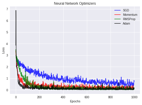
We can see from the plot that Adam and Nesterov Momentum optimizers produce lowest training loss!
References
[1] Ian Goodfellow et. al., “Deep Learning”, MIT Press, 2016.
[2] http://cs231n.github.io/neural-networks-3/
[3] Tensorflow doptimizer documentation
[4] Original Notebook